1800 Words | Approximately 9 Minutes Read | Last Modified on January 1, 0001
Web Site Root
Thomas S. Dye
I am an archaeologist based in Honolulu.
From 2001 to 2018, I owned and operated an archaeological consultancy, T. S. Dye & Colleagues, Archaeologists, where I had the pleasure and privilege of working with very many fine colleagues. With me to the end were my partner, Eric Komori, and two amazing wahine, Muffet Jourdane and Kim Kalama.
I’ve been teaching Hawaiian Archaeology at the University of Hawai`i at Mānoa since 2014.
Starting September 2018, I’m working on a research project with Caitlin Buck and Keith May funded by Historic England. Caitlin is overseeing a PhD student, Bryony Moody, who will write a thesis about automating the process of generating chronological models from digital legacy data.
I’m also working with Anne Philippe at Université de Nantes, Laboratoire de
mathématiques Jean Leray on an R software package, ArchaeoPhases,
which reads the raw MCMC output of Bayesian calibration software such as BCal,
OxCal, and ChronoModel and provides a set of functions to
analyze it.
I’ve developed and released what might be the first open source Harris Matrix
drawing program, hm. I’m using the hm software to investigate the structure and
history of the leeward Kohala field system on Hawai`i Island.
Articles
Posts
Facing a new public
After 17 years promoting myself as an historic preservation service provider to government agencies and private corporations, I now have the wonderful opportunity to pursue my research interests full time. This web site is my way of keeping track of what I’m doing now that my days aren’t filled completing tasks a client requires.
As a firm believer that scientific inquiry and open source software are
inseparable, I’m building my new web presence with an open source tool chain
centered on the Org mode of the Emacs editor. The Org mode sources for the
web page, posts, and projects are exported with Kaushal Modi’s ox-hugo
software and rendered for the web by Hugo.
I intend to add several projects to the two I have at the moment:
- a publications list, with links;
- highlights of a career in cultural resources management;
- tracking progress in the leeward Kohala field system;
- an illustration of the use of
ArchaeoPhasessoftware; and - with some luck, results of a long-dormant project with Jennie Kahn describing the Hawaiian adzes in Bishop Museum.
ArchaeoPhases
In Spring 2016 I took up the opportunity to participate in a two-day conference on Bayesian statistics in archaeology in Nantes, France. Hosted jointly by Philippe Lanos of the Université de Rennes and Anne Philippe at the Université de Nantes, it was a chance to meet and talk with scholars actively working with Bayesian statistics, mostly as archaeologists apply those statistics to dating problems. I was able to catch up with two long-time friends, Caitlin Buck and Bo Meson from Sheffield, and had especially interesting conversations with Andrew Millard from Durham and Frances Healy from Cardiff, whose archaeological work I’d read with interest and admiration.
Philippe and Anne had recently released a Bayesian calibration application,
ChronoModel, that implements a slightly different model than the one Caitlin
implemented in BCal and also used by OxCal. Listening to Anne, Philippe, and
Caitlin discuss the pros and cons of their design decisions helped me make sense
of the high-level statistical papers that describe the decisions. The main
difference is how the models estimate phase boundaries. BCal and OxCal model the
phase boundaries based on an assumption about the distribution of samples within
the phases; ChronoModel doesn’t make the assumption needed to model the phase
boundaries, so it uses the earliest and latest estimates from samples assigned
to the phase. The upshot: don’t expect ChronoModel to agree with BCal or OxCal
on phase boundary estimates—if they do agree, then it is simply a matter of
chance. Also, if the chronological model you are building uses phase boundaries
as target events, then do take the time to understand exactly what the phase
boundary estimates are giving you.
I learned about ArchaeoPhases during the conference dinner when the discussion
turned to the open source statistical software application, R. Anne was excited
by Shiny, an R package for designing interactive web applications. I agreed with
her that applications created with it might help archaeologists gain access to
the statistical power of R.
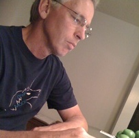
More exciting for me was learning that ArchaeoPhases included an improved
version of the Tempo plot, which I had recently developed as an open source
software project. My version of the Tempo plot assumed a normal approximation
throughout, which made it easy to implement in R and didn’t tax my limited grasp
of mathematics. Anne used her considerable mathematics skills to put the Tempo
plot on a firmer Bayesian footing. The ArchaeoPhases user can now choose between
the normal approximation and the full Bayesian treatment when calling the
TempoPlot function. Check it out!
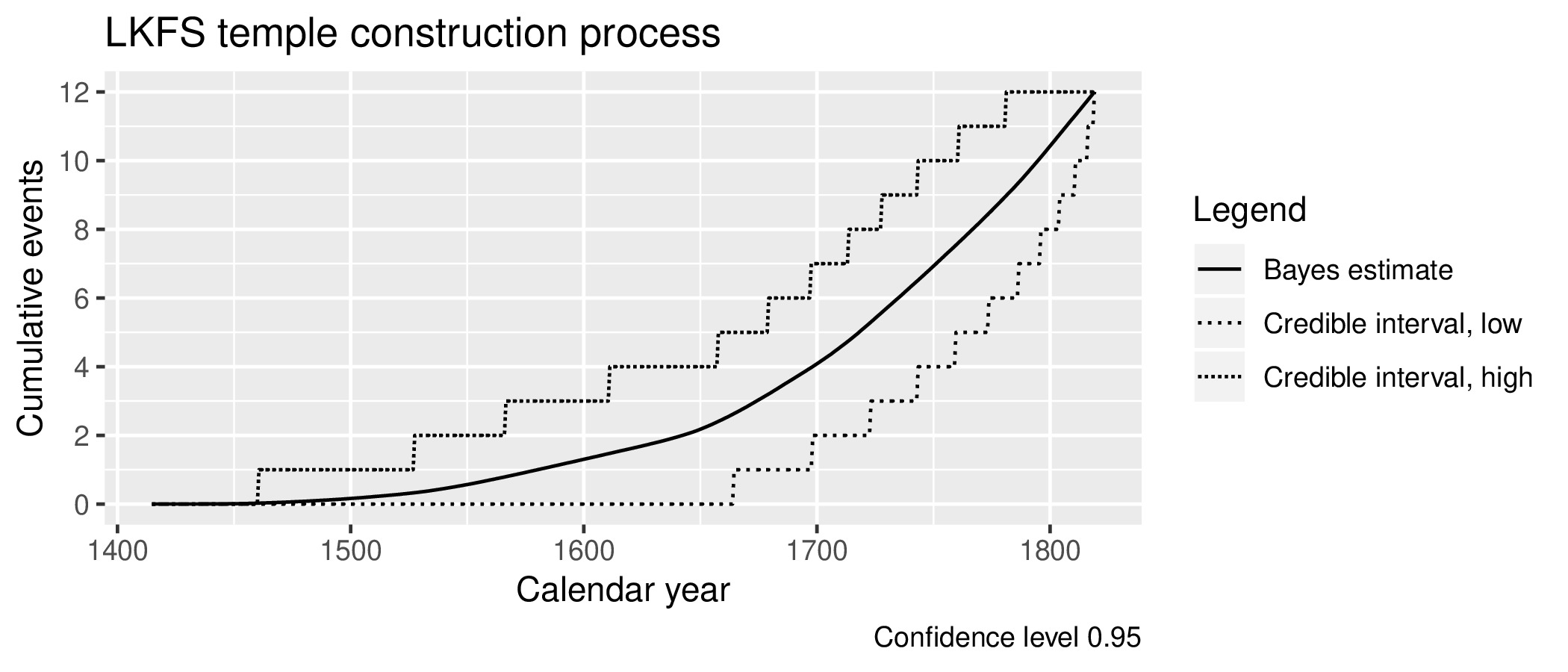
Figure 1: Example of a Tempo plot with the full Bayesian treatment.
Release Early and Often
This is a story about open source software development in archaeology and an example of practicing the software development philosophy known as “release early, release often”.
Back in the early 1990’s, I was exploring the possibility of interpreting a collection of radiocarbon dates as a process, rather than as a collection of events. Eric Komori and I had assembled a database of radiocarbon dates from Hawaiian archaeological sites and were keen to use the database to join a debate over the size of the Contact-era Hawaiian population. We had read a paper by John Rick at Stanford that suggested the idea of using “dates as data.” We thought Rick’s idea could be applied to our database to yield a population growth curve whose shape might contribute to the debate.
At the time, the best practice seemed to be summing the marginal posteriors
yielded by Calib, an approach that eventually generated a large literature and
that archaeologists continue to refine and develop.
As I was working on what to do with the summed marginal posteriors, I had the good sense to ask Caitlin Buck for advice. Caitlin responded that I wasn’t really interested in the marginal posteriors! She claimed I was really interested in properties of the joint posteriors and suggested that I shouldn’t waste my time summing the marginal posteriors in order to infer properties of the joint posteriors. Better, she advised, to investigate the joint posteriors directly.
If I remember correctly, it took me quite a while to think through Caitlin’s
suggestion. First, I had to convince myself that the path Eric and I had chosen
was not the best path. This was hard! Eric and I had written a little computer
program for summing the marginal posteriors reported by Calib and plotting what
we called “annual frequency distribution diagrams.” We were excited that our
program seemed to give us the processual view we were after. I was busy working
on the next step, which we saw as the problem of how to compare annual frequency
distribution diagrams to determine whether or not they were different from one
another. We had worked so hard and the end seemed so close!
Then one day, Caitlin’s insight “clicked” and I was able to see that inferring properties of the joint posteriors by summing marginal posteriors was like reaching behind your head to scratch your ear—it worked, after a fashion, but it was far from the best way to proceed. When Caitlin’s insight “clicked” I could see how to use the Markov chain/Monte Carlo (MCMC) engine at the heart of Bayesian calibration software to investigate the joint posteriors. I had the outline of an algorithm to produce what I would later come to call a tempo plot, but at the time there was no easy access to an MCMC engine, and with life’s contingencies pressing in, I filed the project away with the hope that someone else would take it up and save me some work.
Fast forward a decade and a half and I’ve engaged a debate on the tempo of change in old Hawai`i in the centuries leading up to Captain Cook’s visit in 1778–1779. Figure 1 in that paper summarizes the marginal posteriors, and works after a fashion to carry the argument of the paper, but it would have been better as a tempo plot. It was time to revisit Caitlin’s suggestion.
A survey of the field yielded a couple of interesting data points:
- Bayesian calibration applications now gave access to the MCMC engine with an option to write out its internal state during calculations; and
- archaeologists had shown just a bit of interest in joint posteriors and no one had worked out a procedure for producing a tempo plot.
Implementing the initial version of the tempo plot in R was relatively quick and
easy. As I began to use the tempo plot to explore dating evidence from Hawai`i,
I soon found that the processes associated with different kinds of events had
distinct shapes. Eventually, I distinguished three shapes, which I associated
with processes of tradition, fashion, and innovation and referred to as
long-term rhythms in the development of Hawaiian social stratification. The R
source code I’d developed was released as supplementary material for the
published paper—release early!
Through a bit of serendipity and good fortune, Anne Philippe at Université de
Nantes, Laboratoire de mathématiques Jean Leray saw the paper and built the
tempo plot into an R software package, ArchaeoPhases, which reads the raw MCMC
output of Bayesian calibration software such as BCal, OxCal, and ChronoModel and
provides a set of functions to analyze it. This was a big improvement in two
senses:
- Anne did more than just include my code in
ArchaeoPhases. She also used her considerable mathematics skills to put the Tempo plot on a proper Bayesian footing so the user can choose between the normal approximation and a full Bayesian treatment; and - publishing
ArchaeoPhaseson the Comprehensive R Archive Network established a version control space that automates the release process—it was now possible to release often!
Since that time, the tempo plot has been revised to give the user lots of
control about how the plot looks. Figure 2 shows a tempo plot
gussied up for a dark-themed slide show. Figure 3 shows the same tempo
plot presented in the style of Edward Tufte. Check out the current ArchaeoPhases
release!
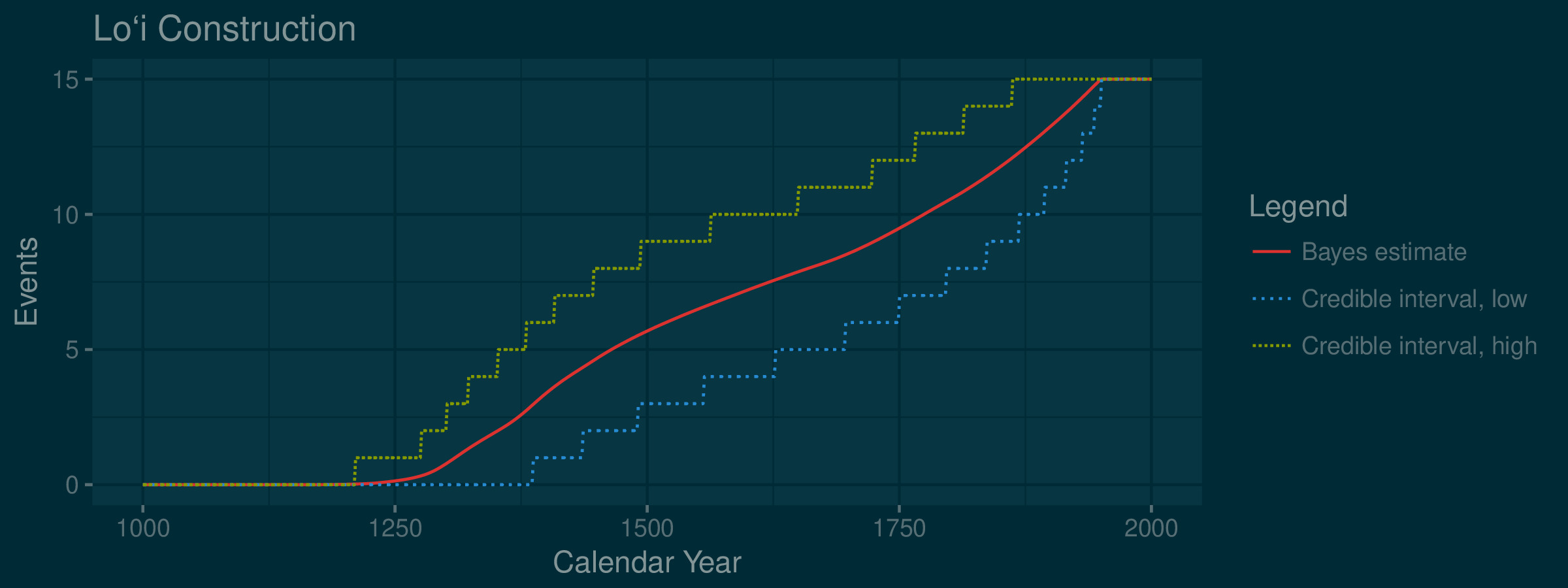
Figure 2: The tempo of pondfield construction plotted on a dark background for a slideshow.
Figure 3: The tempo of pondfield construction plotted in the style of Edward Tufte.
Here is the takeaway: releasing early and often fosters collaboration and progress.