Bayesian Inference for Archaeologists
Thomas S. Dye (tdye@hawaii.edu)
30 November 2018
Public Availability
The slides for this lecture are publicly available:
http://tsdye.online/bayes/bayesian-inference.html
Bayes' Rule
In plain English: "The posterior probability is proportional to the product of the likelihood and the prior probability."
The Basis of Bayes' Rule
Bayes' rule is based on a transitivity condition, a sum rule, and a product rule.
Transitivity Condition
Given three propositions, A, B, and C
- if we believe A more than B
- and we believe B more than C
- then we must necessarily believe A more than C
Sum Rule
- Expressing a belief that something is true, \(p(X)\)
- is an implicit expression of the belief that it might be false, \(p(\bar{X})\)
\(p(X) + p(\bar{X}) = 1\)
Product Rule
- Expressing a belief that (proposition) \(Y\) is true, \(p(Y)\)
- and that \(X\) is true given that \(Y\) is true, \(p(X|Y)\)
- is an implicit expression of a belief that both \(X\) and \(Y\) are true, \(p(X,Y)\)
\(p(X,Y) = p(X|Y) \times p(Y)\)
Derive Bayes' Rule
Bayes' Rule is a consequence, or corollary, of the sum and product rules and the transitivity condition. Three algebraic steps derive Bayes' Rule. An additional step yields a simplified version.
First Step
Transpose \(X\) and \(Y\) in the product rule:
\(p(X,Y) = p(X|Y) \times p(Y)\)
\(p(Y,X) = p(Y|X) \times p(X)\)
Second Step
Note that \(p(Y,X) = p(X,Y)\):
\(p(X|Y)\ \times\ p(Y) = p(Y|X)\ \times\ p(X)\)
Third Step
Divide through by \(p(Y)\) to get Bayes' Rule:
\[p(X|Y) = {p(Y|X)\ \times\ p(X) \over p(Y)}\]
A Simplified Form
Eliminate the denominator on the right hand side and replace the equality sign with a sign of proportionality:
\(p(X|Y) \propto p(Y|X) \times p(X)\)
Brief History of Bayesian Statistics
The 250 year history of Bayesian statistics
- started with an idea
- waited 150 years for philosophical grounding
- developed mathematically for 50 years
- experienced explosive growth in the age of computers
Philosophy and Mathematics
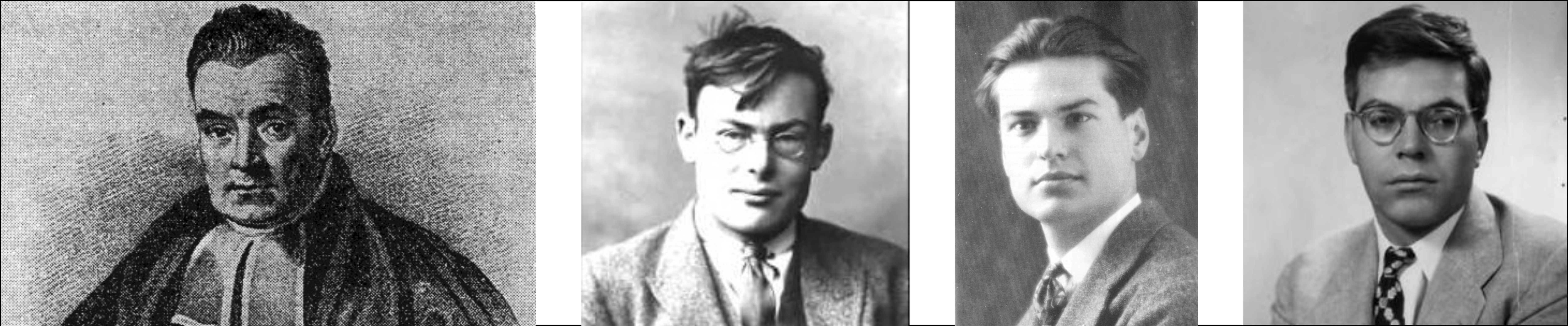
Figure 1: Left to right: Rev. Thomas Bayes (1702–1761), Frank P. Ramsey (1903–1930), Bruno de Finetti (1906–1985), Leonard J. Savage (1917–1971).
Statistics and Archaeology
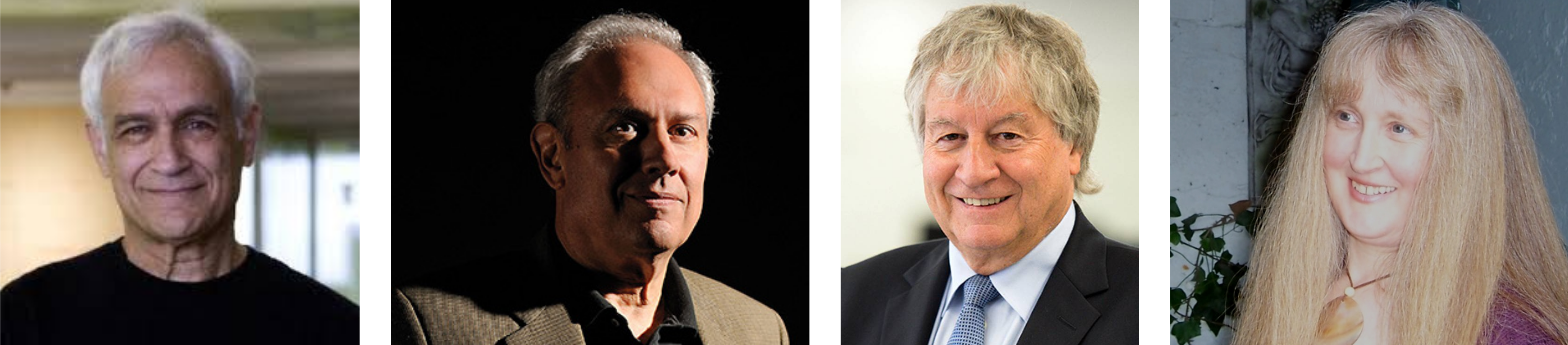
Figure 2: Left to right: Stuart Geman (1949–), Donald Geman (1943–), Sir Adrian Smith (1946–), Caitlin Buck (1964–)
Bayesian Bible for Archaeologists
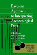
Figure 3: Buck, C. E., W. G. Cavanagh, and C. D. Litton (1996) Bayesian Approach to Interpreting Archaeological Data. John Wiley & Sons, New York, NY.
Bayesian Calibration Applications
Three Bayesian calibration applications are freely available.
BCal
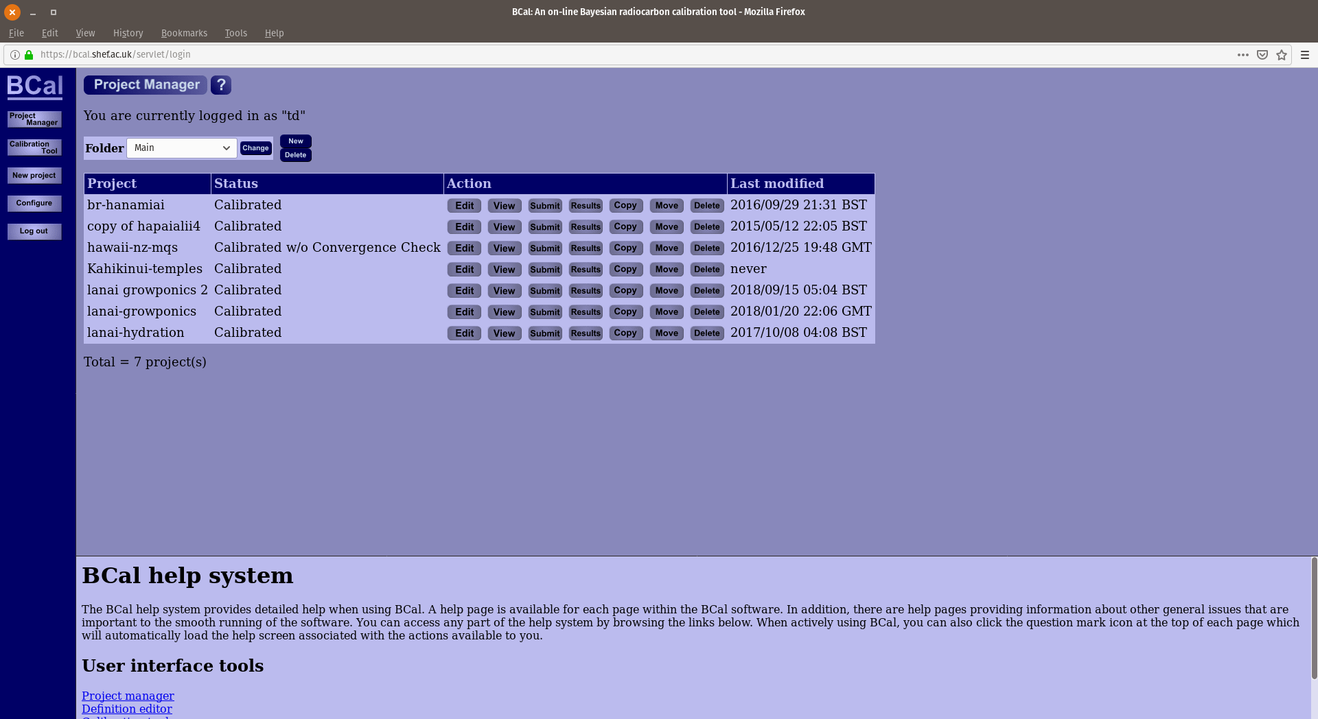
Figure 4: https://bcal.shef.ac.uk/top.html
OxCal
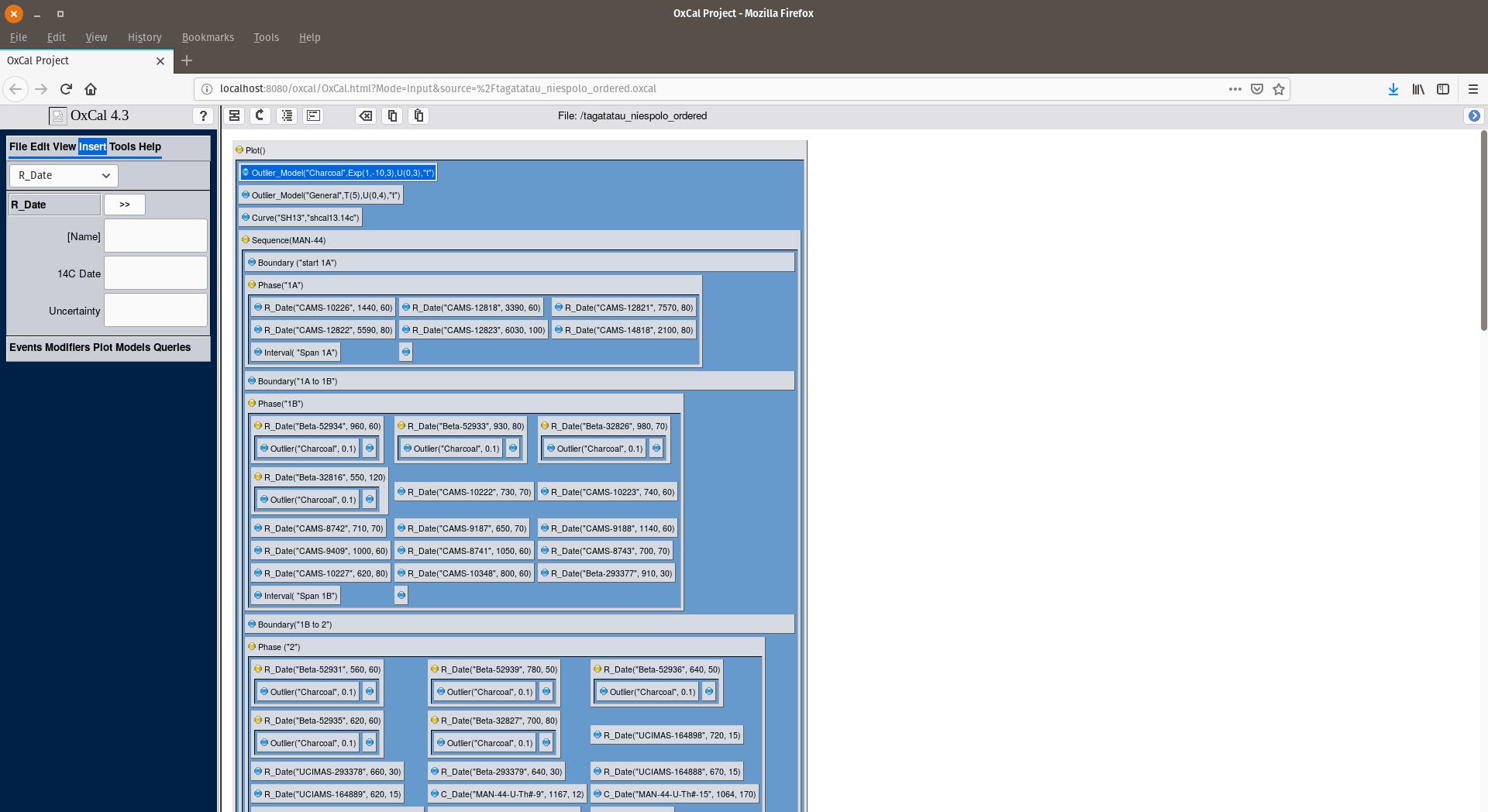
Figure 5: https://c14.arch.ox.ac.uk/oxcal.html
ChronoModel
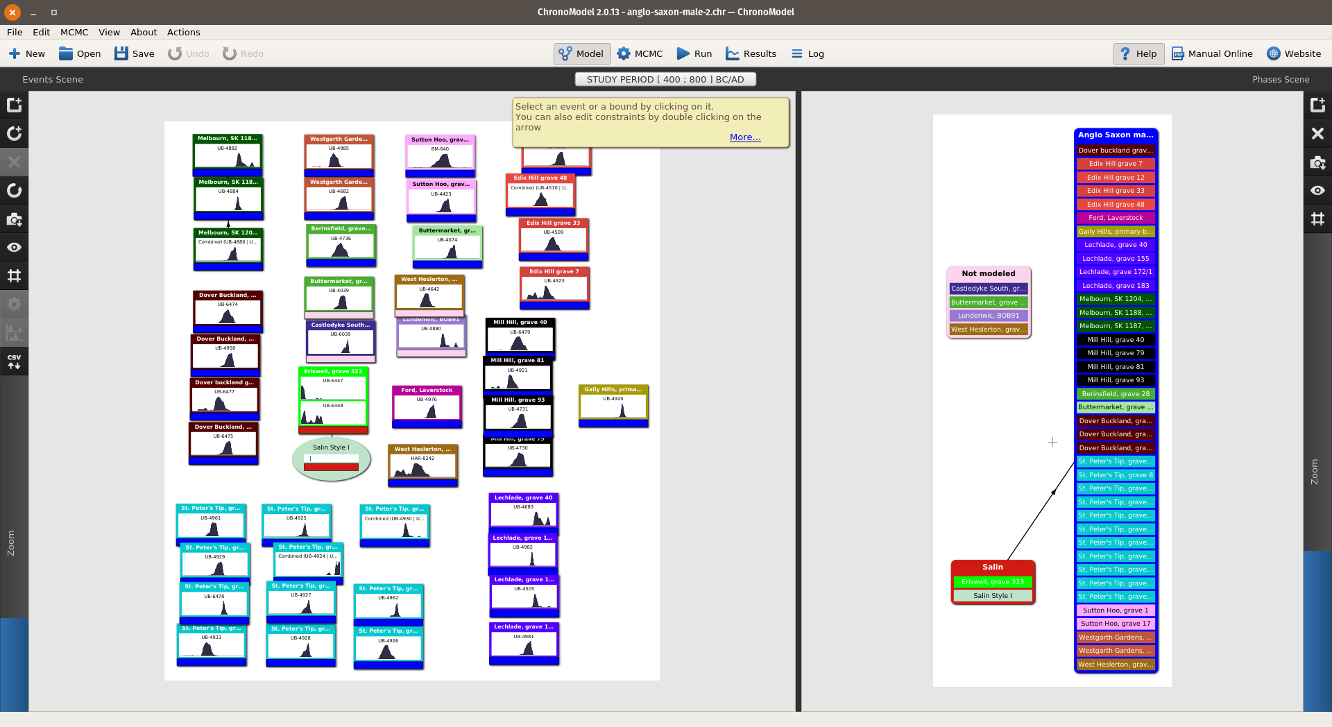
Figure 6: https://chronomodel.com/
How Bayesian Calibration Works
This schematic overview of the priors, data, likelihoods, and posteriors glosses over many details that can be found in Buck, Cavanagh, and Litton's book, Bayesian Approach to Interpreting Archaeological Data.
Prior Information
Bayesian inference recognizes that an archaeologist brings knowledge and beliefs to an inquiry. Bayesian calibration organizes this prior information in terms of phases and events. By convention:
- the start date of Phase n is represented as αn
- the end date of Phase n is represented as βn
- the calendar age of Event i is represented as θi
The Chronological Model
A chronological model specifies what is known and believed about the relative ages of the events and phases. Here is a simple model with two phases and two events, where > means "is older than" and = means "is the same age as":
αa > θ1 > βa = αb > θ2 > βb
Stratigraphy as Prior Information
αa > θ1 > βa = αb > θ2 > βb
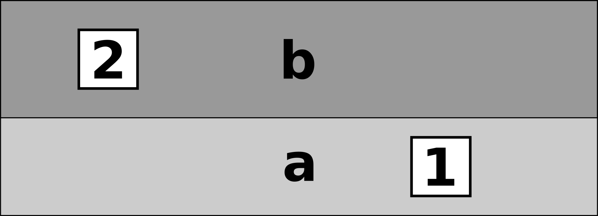
Figure 7: Stratigraphic section showing contexts a and b and objects 1 and 2.
Sources of Data
Bayesian calibration can model most sources of chronological information that might be used to estimate the age of events.
- \(^{14}\)C age estimates
- thermoluminescence age estimates
- archaeomagnetic age estimates
- \(^{230}\)Th and other age estimates whose errors are normally distributed
- any artifact reliably assigned to a temporally sensitive class
Example of Inverted Age Estimates
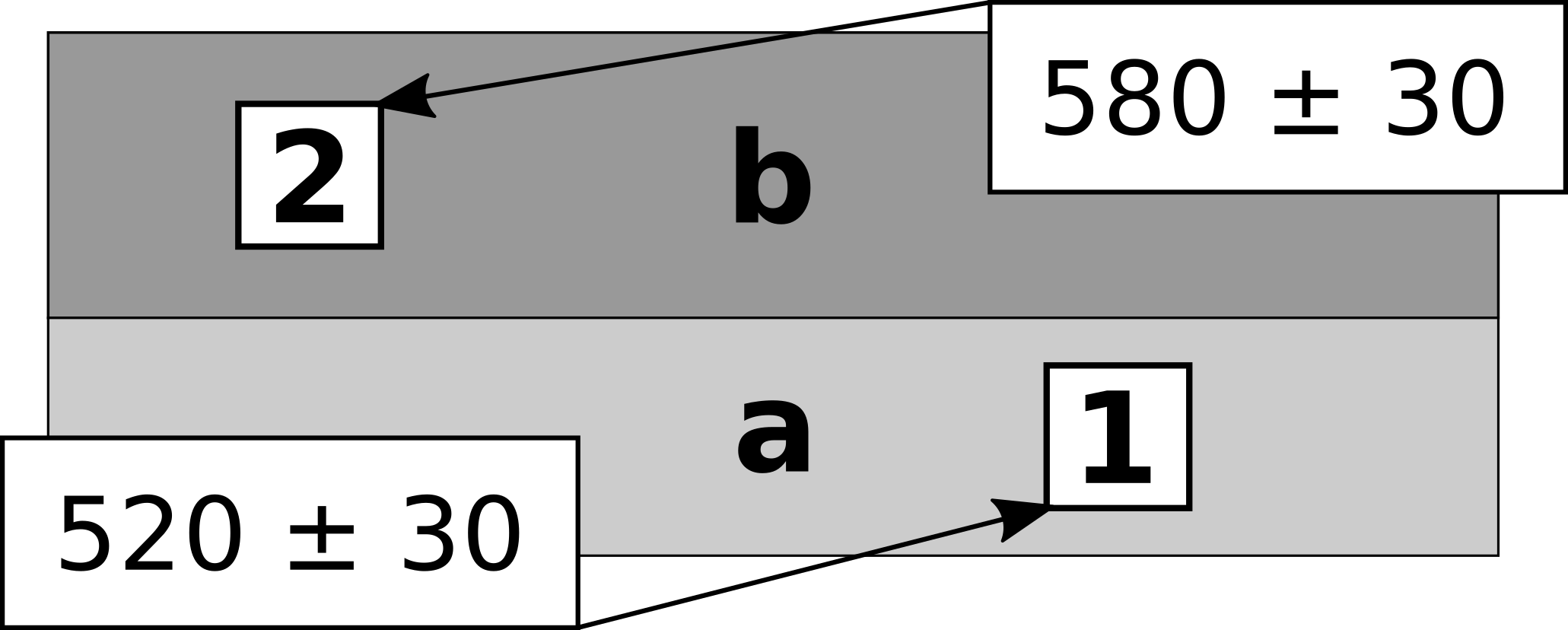
Figure 8: Age estimates for the events associated with objects 1 and 2. Note the inversion.
Model Yields Interpretable Results
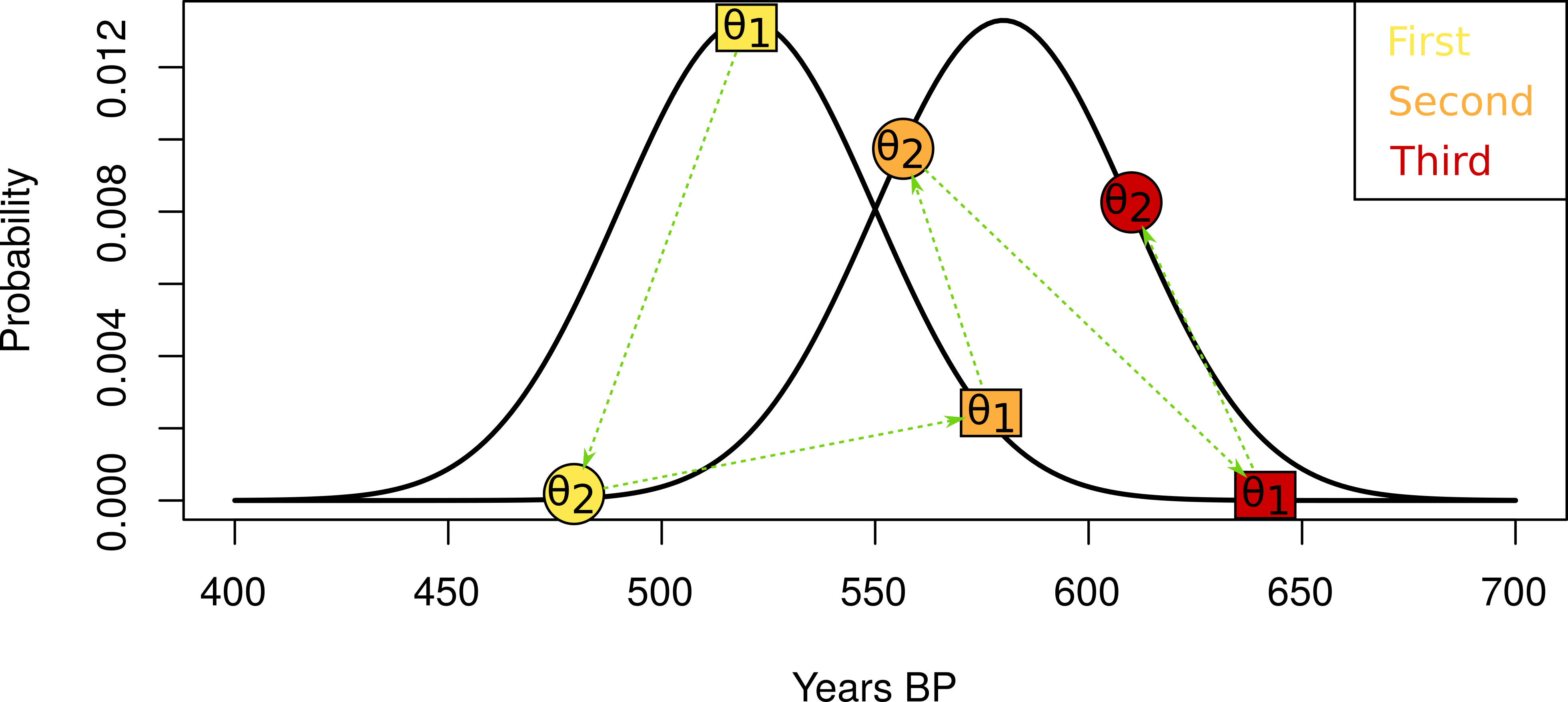
Figure 9: Hypothetical Markov Chain Monte Carlo process at the heart of Bayesian calibration.
Implementation in Chronomodel
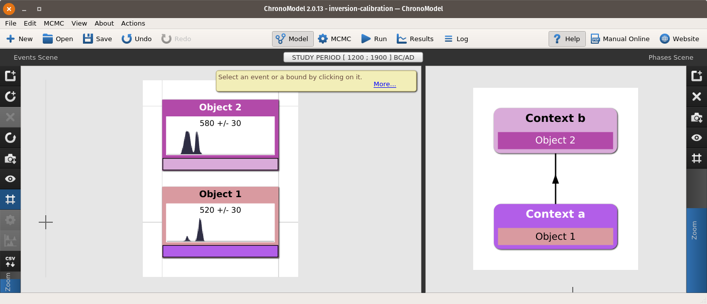
Figure 10: The inverted age estimates modeled in Chronomodel 2.0.13.
Calibration Results
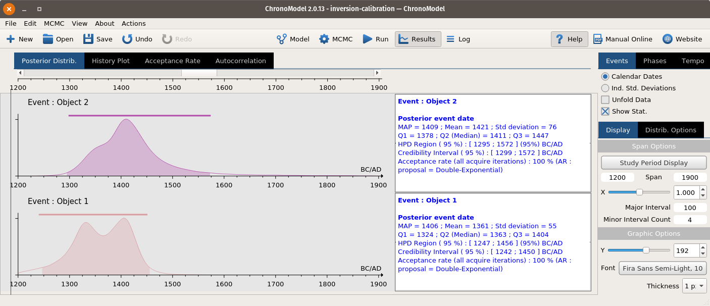
Figure 11: The results of Bayesian calibration are archaeologically interpretable.
Interpreting Bayesian Posteriors
Bayesian posteriors can be interpreted as events, occurrences, and processes with the ArchaeoPhases software.
ArchaeoPhases as a Shiny Application
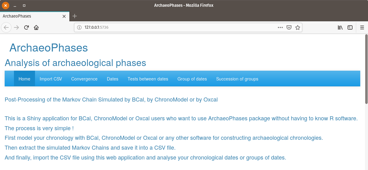
Figure 12: The ArchaeoPhases R package running as a Shiny application.
Interpreting Posteriors as Events
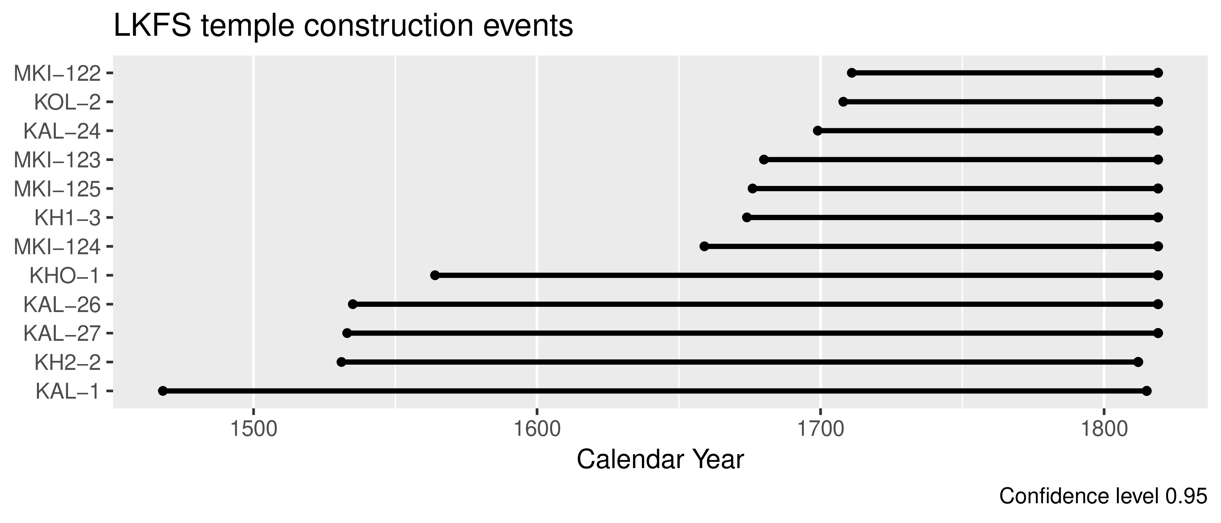
Figure 13: Temple construction events in the leeward Kohala field system.
Interpreting Posteriors as Occurrences
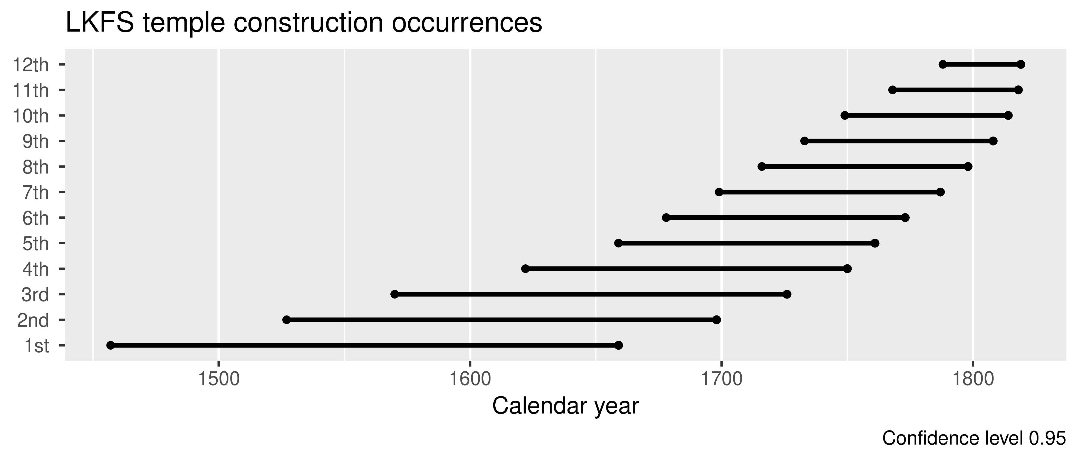
Figure 14: Additions to the system of temples in leeward Kohala.
Interpreting Posteriors as a Process
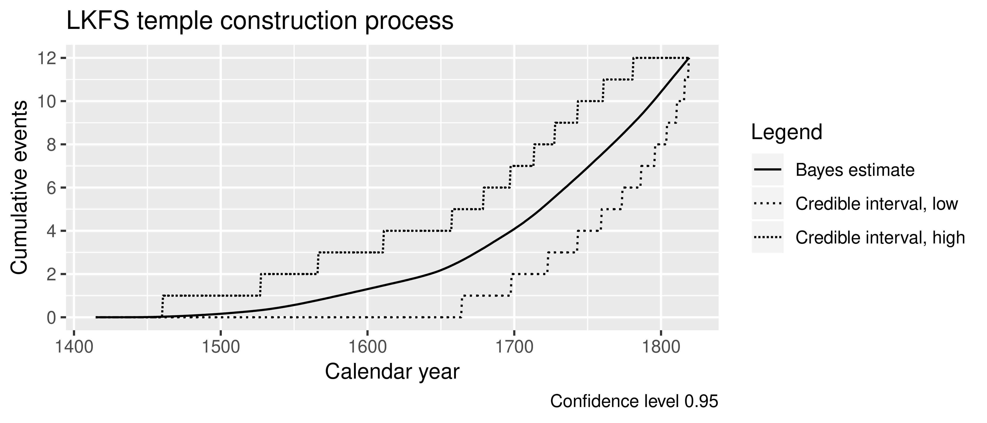
Figure 15: Tempo of change in the leeward Kohala system of temples.
Operationalizing Processualism
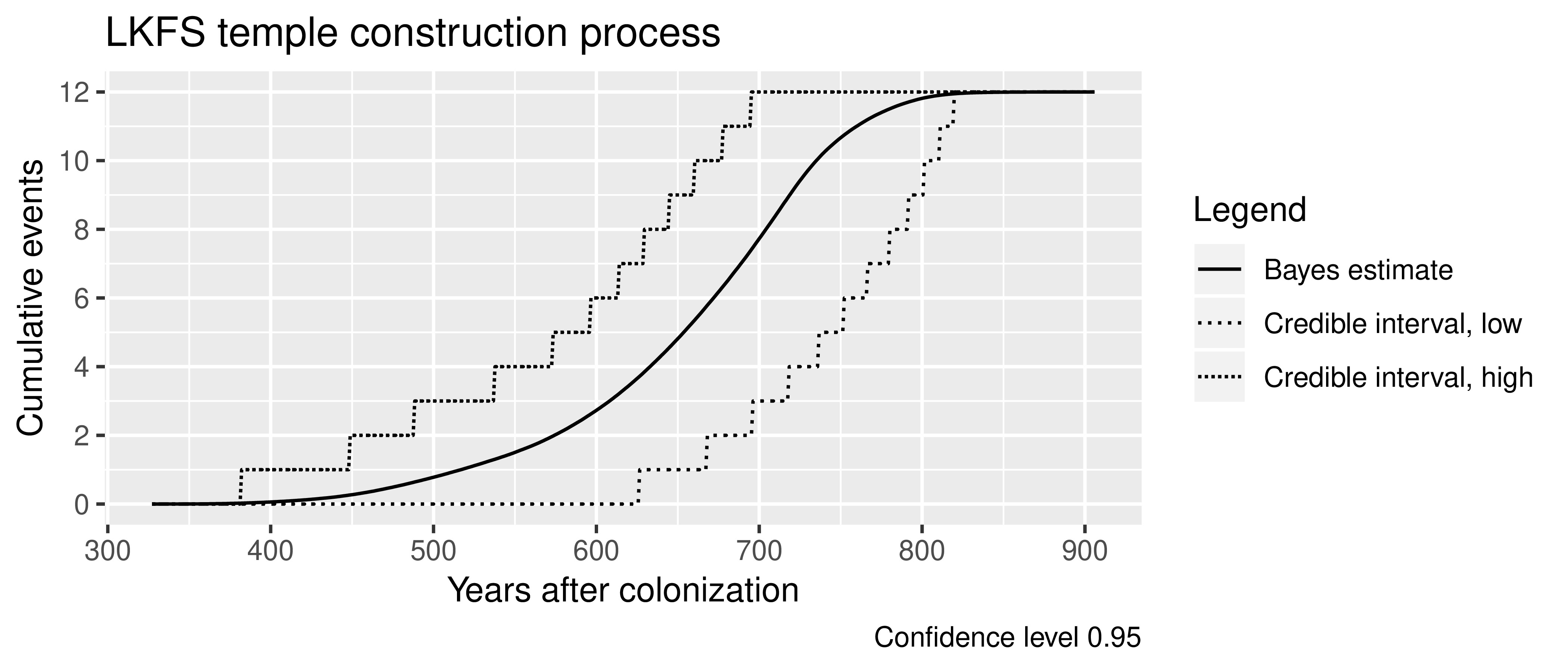
Figure 16: A processual view of change in old Hawai`i.